
This blog introduces our paper Beyond Quadratic Loss: The Stability Phase Diagram of Adam, which addresses three main questions:
- How do Adam’s beta settings determine whether training is smooth or exhibits recurring loss spikes?
- What do the boundaries between these phases tell us about the loss landscape?
- Why does this loss landscape arise naturally in confident cross-entropy (CE) training?
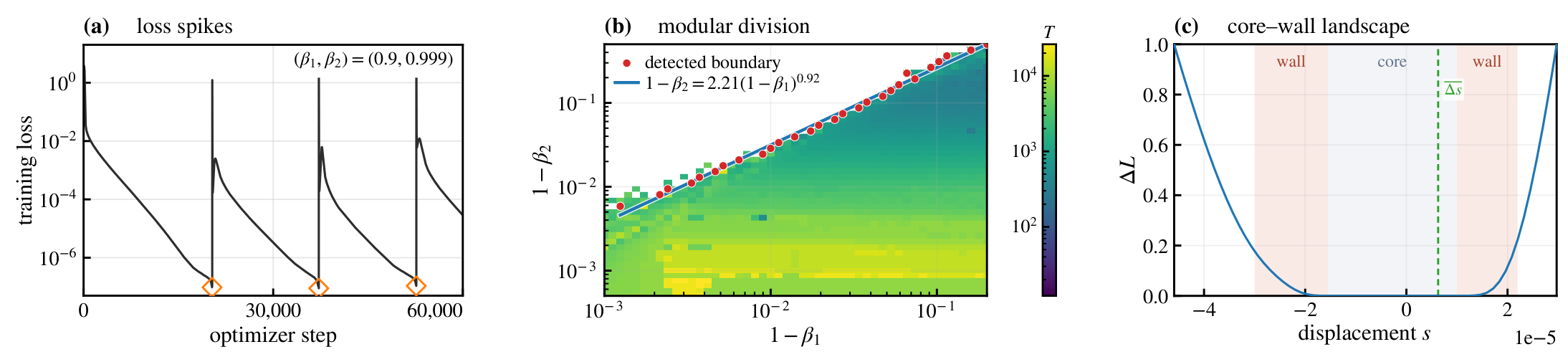
Figure 1 · Adam loss spikes, phase diagram, and core–wall landscape
The figure above gives the full picture of this work. (a) A Transformer trained on modular division exhibits recurring loss spikes. Orange diamonds mark the low-loss points before spikes. (b) Across \((\beta_1,\beta_2)\) settings, a clear phase boundary separates spiky from smooth training, with color indicating the oscillation period. (c) The pre-spike loss landscape has a narrow core and a steep wall. The green dashed line marks the typical update scale.
How do Adam’s beta settings determine whether training is smooth or exhibits recurring loss spikes?
Adam’s \(\beta_1\) and \(\beta_2\) control the memory timescales of the first and second gradient moments, respectively. As they approach 1, these timescales grow, approximately as \(1/(1-\beta_1)\) and \(1/(1-\beta_2)\). The interplay between these two timescales governs whether macroscopic loss spikes recur during training.
We present the first systematic observation of Adam’s phase boundary across beta settings in real-model training. We train six model–task settings with AdamW: Transformers for modular division and modular addition, a character-level Transformer for Tiny Shakespeare, an MLP and a CNN for CIFAR-10, and an MNIST autoencoder. Varying only \(\beta_1,\beta_2\) within each setting reveals a near-linear boundary between spiky and smooth training:
\[1-\beta_2\simeq C(1-\beta_1).\]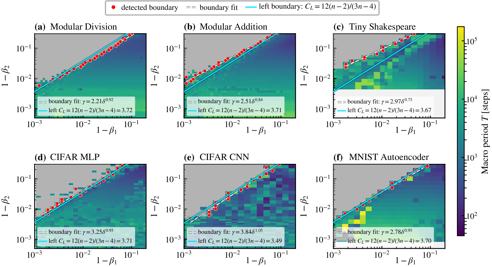
Figure 2 · Adam phase diagrams across six model–task settings
Red points mark the phase boundary, and white dashed curves show power-law fits. At fixed \(\beta_1\), larger \(\beta_2\) lies on the spiky side, and the oscillation period grows as \(\beta_2\) approaches 1. This shared pattern across different models identifies the relative memory timescales as a key to understanding Adam spikes.
What do the boundaries between these phases tell us about the loss landscape?
To understand this pattern, we first run Adam on a one-dimensional quadratic loss, then replace it with a superquadratic power-law loss. The two produce markedly different scaling:
\[\begin{aligned} L(x)\propto x^2 &: \quad 1-\beta_2\propto(1-\beta_1)^3,\\ L(x)\propto |x|^n,\quad n>2 &: \quad 1-\beta_2\propto(1-\beta_1). \end{aligned}\]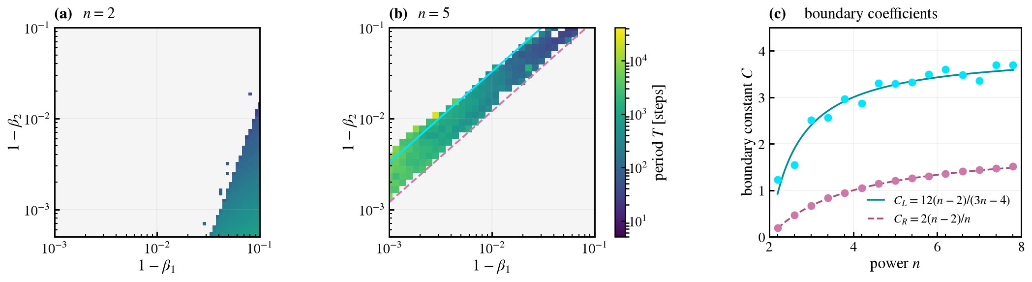
Figure 3 · Phase boundaries for quadratic and superquadratic losses
Panels (a) and (b) correspond to \(n=2\) and \(n=5\), respectively, while (c) shows how the boundary coefficients vary with \(n\). The near-linear phase boundary in real models points to a non-quadratic loss landscape at the scale of an Adam update.
Examining real-model loss slices along the Adam-preconditioned gradient direction reveals a core–wall landscape: a flat, narrow quadratic core, a steep superquadratic wall outside it, and an outer rollover where growth slows. As training progresses, the core contracts toward the typical update scale. Adam begins to explore the wall and encounters a large effective loss exponent. Panel (c) of the opening figure illustrates this geometry.
We measure the effective wall exponent \(n\) at pre-spike points, obtaining values of approximately \(6.5\)–\(10.9\) across the six settings. Substituting these values into the toy model’s empirical relation
\[C_L(n)\simeq\frac{12(n-2)}{3n-4},\]estimates the scale of the phase-boundary coefficients in real models. The cyan lines in the six-model figure show these estimates, directly connecting the loss landscape to the phase diagram across beta settings.
Why does this loss landscape arise naturally in confident CE training?
Confident CE describes a training regime in which the model is highly confident in the correct answers. The logit margins between correct and incorrect classes are large, and the loss is low. Let \(y_i\) be the correct class for sample \(i\), and let \(m_{ij}(s)\) be its margin over an incorrect class \(j\), where \(s\) is displacement along a fixed parameter direction. Locally expanding the margin as \(m_{ij}(s)\simeq m_{ij}-a_{ij}s\) gives an exponential-sum approximation to CE:
\[\begin{aligned} L_{\rm CE}(s)&=\frac{1}{N}\sum_i\log\left(1+\sum_{j\ne y_i}e^{-m_{ij}(s)}\right),\\ L_{\rm conf}(s)&\simeq\frac{1}{N}\sum_i\sum_{j\ne y_i}e^{-m_{ij}+a_{ij}s}. \end{aligned}\]Here, \(N\) is the number of samples, and \(a_{ij}\) describes how the margin changes along this direction. Large positive margins suppress the loss through \(e^{-m_{ij}}\), while displacement amplifies some contributions through \(e^{a_{ij}s}\), causing the loss to rise rapidly. The flat core and steep wall arise naturally from the exponential structure of confident CE.
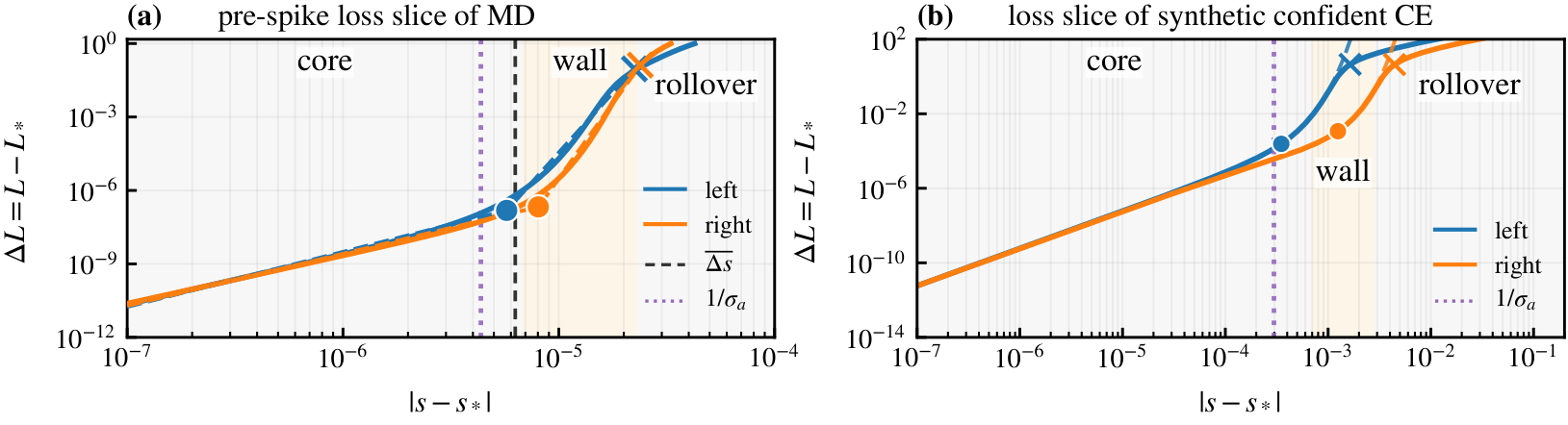
Figure 4 · Core–wall landscapes in a real model and confident CE
The left panel shows a real-model loss slice before a spike, and the right panel is constructed directly from synthetic confident CE. Both exhibit a core, a wall, and a rollover. Under a Gaussian approximation to the CE-weighted distribution of directional margin slopes, its width \(\sigma_a\) sets the quadratic-core scale: \(s_{\rm core}\sim1/\sigma_a\). Beyond the core, rapidly growing exponential terms produce a superquadratic wall. At larger displacements, the logarithm in exact CE slows the growth, producing the rollover.
For the real model in the left panel, \(1/\sigma_a\simeq4.35\times10^{-6}\), while the typical update is approximately \(6.3\times10^{-6}\). A single update can cross the quadratic core and reach the steep wall. This connects the form of confident CE, finite-scale loss geometry, and Adam’s training phases through a complete mechanism.
Outlook
This work raises two natural questions:
- Can an optimizer estimate the effective loss exponent at its own update scale and use it to adjust the learning rate or \(\beta_1,\beta_2\)?
- How do margins and their directional slopes evolve during training, driving core contraction and progressive sharpening at finite scales?