
This blog offers a quick overview for newcomers to quantum error correction (QEC) decoders. It is based on my October 9 talk at the quantum theory discussion group at the Institute for Interdisciplinary Information Sciences (IIIS) and covers three topics: conventional decoders, machine learning decoders, and online decoding. The slides (PDF) are available for download.
1. The decoder’s task
Let us first establish three terms. A mechanism is a candidate error mechanism together with its binary variable. The literature also calls it an error, error mechanism, or variable. \(x_i=1\) means that mechanism \(i\) occurs, while \(x_i=0\) means that it does not. The vector \(x\) specifies the configuration of all mechanisms, and \(p_i\) is the prior probability of mechanism \(i\).
A detector is a check quantity used to detect errors. In repeated syndrome extraction, it is typically the modulo-2 difference between consecutive syndrome measurements of the same stabilizer. If \(m_{c,t}\) is the syndrome measurement for stabilizer \(c\) in round \(t\), then \(s_{c,t}=m_{c,t}\oplus m_{c,t-1}\). \(s_a=1\) means that detector \(a\) is triggered, while \(s_a=0\) means that it is not. The vector \(s\) contains all detector values. Throughout this blog, a detector event or detection event is described as a “triggered detector.” A logical is a tracked logical observable. \(\ell_\alpha=1\) means that logical \(\alpha\) is flipped, and \(\ell\) is the vector of all logical flips.
The effects of mechanisms on detectors and logicals are described by binary linear maps \(H\) and \(A\), respectively. Over \(\mathbb F_2\),
\[Hx=s,\qquad \ell=Ax.\]Consider a decoder that outputs a mechanism configuration. It takes \(p,s,H\) as input and seeks a configuration \(\hat x\) satisfying \(H\hat x=s\). Satisfying the detector constraints only means that the configuration explains the observations. Successful correction additionally requires \(A\hat x=\ell\): the predicted logical flips must match the actual ones. Throughout this blog, \(d\) denotes the code distance, and \(s\) denotes the detector vector.
\(H\) also defines an undirected bipartite graph called the Tanner graph. Each row corresponds to a detector node, each column to a mechanism node, and \(H_{ai}=1\) indicates an edge between them. For a low-density parity-check (LDPC) code, this graph is sparse. Many high-performance quantum LDPC (qLDPC) code constructions use expander properties and have nonlocal connectivity that is difficult to realize using only local connections in two dimensions. For constraints that connectivity imposes on code performance, see baspin2021.
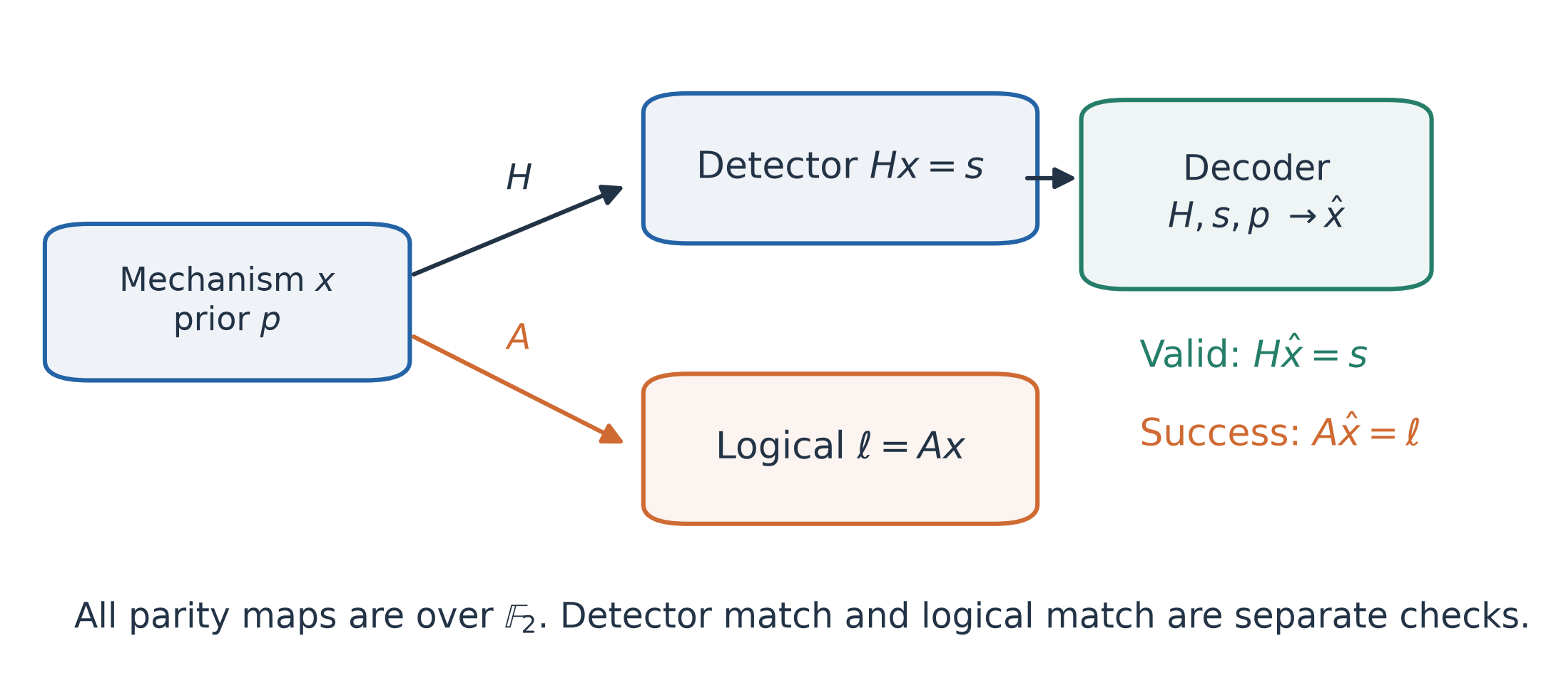
Figure 1 · Decoder inputs and objectives
The noise model determines which mechanisms we use. Circuit-level noise describes specific faults in the circuit, such as a Pauli Z caused by idle dephasing, or single-qubit and two-qubit errors in a two-qubit gate. Phenomenological noise considers only data mechanisms and measurement mechanisms, representing data errors and measurement errors, respectively. Errors across multiple correction rounds are grouped into these two categories.
At fixed \(s\), mechanism configurations producing the same \(\ell\) belong to the same logical class. Decoding therefore has two distinct objectives: finding an approximately minimum-weight mechanism configuration, or finding the logical class with the largest total probability. Most minimum weight perfect matching (MWPM), belief propagation (BP), and beam search methods focus on the former. The latter requires summing the probabilities of multiple configurations within each logical class. It accounts for degeneracy in quantum error correction, but is usually harder to implement.
2. Conventional decoders
This section introduces MWPM, BP and its post-processing methods, and Tesseract. Tesseract achieves logical error rates at the state of the art, but is relatively slow. RelayBP is faster, with somewhat lower accuracy.
Personal view. In my view, taking Tesseract as a reference, classical decoders have relatively limited room for further accuracy improvements. Comparing the likelihoods of decoded and actual configurations shows that, in most failed samples, the decoded configuration has the higher likelihood. In other words, even finding the most likely configuration cannot correct such errors. More effort can therefore go toward reducing decoding time. One approach is to combine decoders in stages: start with a weaker but faster decoder, then send samples that fail to decode or yield questionable results to a stronger but slower decoder, escalating through further stages as needed. At low physical error rates, errors in most shots are local and can be handled by a few BP iterations. Only a small fraction of difficult configurations need a more complex decoder. The telescoping decoder in the Mitten codes paper follows this approach bhardwaj2026.
Minimum weight perfect matching
MWPM is fast and finds a minimum-total-weight solution within the matching model. Sparse Blossom is a representative efficient implementation higgott2025. MWPM requires each mechanism to affect at most two detectors, making it suitable for graphlike decoding in surface codes, but generally preventing its direct application to most qLDPC codes.
In this model, each mechanism is a weighted edge connecting detectors. A mechanism affecting only one detector can connect to a boundary. Multiple mechanisms form paths, with triggered detectors at their endpoints. Decoding can therefore be formulated as pairing the triggered detectors.
For a given detector pair, the most likely configuration \(x\) corresponds to a minimum-total-weight path between them. One can therefore first compute shortest-path distances between triggered detectors to construct a matching graph, then use the Blossom algorithm to select the pairing with the smallest total weight.
Let \(k\) be the number of currently triggered detectors, \(n\) the total number of nodes in the detector graph, and \(m\) its number of edges. An upper bound on the complexity of “shortest-path preprocessing + matching” is
\[O\!\left(k(m+n)\log n+k^3\right).\]Sparse Blossom works directly on the sparse detector graph, avoiding this shortest-path preprocessing. In the paper’s low-error-rate benchmarks, the observed runtime grows approximately linearly with problem size.
Belief propagation
BP operates on the Tanner graph defined by \(H\). The input priors \(p\) and detector observations \(s\) reside on mechanism and detector nodes, respectively. BP passes scalar messages between the two node types, incorporating information from \(s\) into the estimates of individual mechanisms to obtain posterior probabilities. For a related introduction, see liu2019.
Below, \(i,j\) index mechanism nodes, \(a,b\) index detector nodes, \(N(\cdot)\) denotes a neighborhood, and \(t\) is the iteration index.
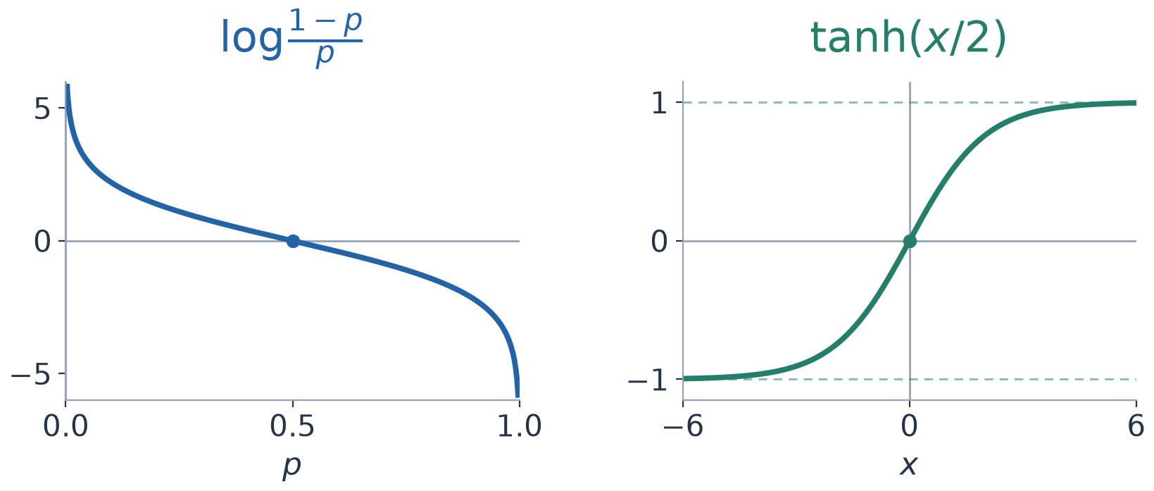
Figure 2 · Tanh and atanh in BP updates
-
Initialize. Compute each mechanism’s prior log-likelihood ratio (LLR) from its prior probability, and initialize mechanism → detector messages:
\[L_i=\log\frac{1-p_i}{p_i},\qquad q_{i\to a}^{(0)}=L_i.\] -
Update detector → mechanism messages. Detector \(a\) uses messages from its other neighboring mechanisms to tell \(i\) what is needed to satisfy the detector constraint:
\[r_{a\to i}^{(t)}=2\operatorname{atanh}\!\left[(-1)^{s_a}\prod_{j\in N(a)\setminus\{i\}}\tanh\!\left(\frac{q_{j\to a}^{(t-1)}}2\right)\right].\]The observed detector value enters the update through \((-1)^{s_a}\).
-
Update mechanism → detector messages. Add the prior LLR to messages from the other detectors:
\[q_{i\to a}^{(t)}=L_i+\sum_{b\in N(i)\setminus\{a\}}r_{b\to i}^{(t)}.\]Both updates exclude the recipient, avoiding the immediate return of information just received.
-
Compute the posterior and make a hard decision. The posterior LLR includes messages from all neighbors:
\[M_i^{(t)}=L_i+\sum_{a\in N(i)}r_{a\to i}^{(t)}.\]Convert \(M_i\) into a posterior probability and a hard decision:
\[\widetilde p_i=\operatorname{sigmoid}(-M_i),\qquad \hat x_i=\mathbf 1[M_i<0].\] -
Check the detector constraints. If \(H\hat x=s\), output \(\hat x\). Otherwise, set \(t\leftarrow t+1\) and return to step 2, until the maximum iteration count is reached. Standard BP only needs to carry \(q\) between iterations. The remaining quantities can be computed within the current iteration. For a Calderbank–Shor–Steane (CSS) code, a common approach is to process the X and Z parts separately, obtaining \(\hat x_X\) and \(\hat x_Z\).
RelayBP: changing the iteration dynamics. RelayBP, proposed by IBM, is a strong-performing BP variant. It uses multiple segments of iterations with different memory strengths to mitigate oscillations and trapping sets in standard BP muller2025.
Blue highlights mark the parts that differ from the BP updates above: the dynamic bias, the MinSum update, and the replacement of \(L_i\) by \(\Lambda_i^{(t)}\).
-
Initialize. Use the original prior, setting \(q_{i\to a}^{(0)}=M_i^{(0)}=L_i\).
-
Construct a dynamic bias. Use the previous iteration’s posterior to adjust the current bias:
\[{\color{#0057ff}\boldsymbol{\Lambda_i^{(t)}=(1-\gamma_i)L_i+\gamma_i M_i^{(t-1)}}}.\] -
Update detector → mechanism messages. Use a MinSum update:
\[r_{a\to i}^{(t)}={\color{#0057ff}\boldsymbol{(-1)^{s_a}\prod_{j\in N(a)\setminus\{i\}}\operatorname{sgn}\!\left(q_{j\to a}^{(t-1)}\right)\min_{j\in N(a)\setminus\{i\}}\left|q_{j\to a}^{(t-1)}\right|}}.\] -
Update mechanism → detector messages and the posterior. Replace the original prior LLR with the dynamic bias:
\[q_{i\to a}^{(t)}={\color{#0057ff}\boldsymbol{\Lambda_i^{(t)}}}+\sum_{b\in N(i)\setminus\{a\}}r_{b\to i}^{(t)},\] \[M_i^{(t)}={\color{#0057ff}\boldsymbol{\Lambda_i^{(t)}}}+\sum_{a\in N(i)}r_{a\to i}^{(t)}.\] -
Make a hard decision and check the detector constraints. Form the hard decision \(\hat x_i=\mathbf1[M_i<0]\), then check \(H\hat x=s\) and record the candidate if it satisfies the constraints. If the current leg needs further iterations, set \(t\leftarrow t+1\) and return to step 2. When \(\gamma_i=0\), these updates reduce to MinSum-BP.
“Relay” means splitting the iterations into multiple legs. Within each leg, the \(\gamma_i\) values are fixed and may differ across mechanisms. Subsequent legs change these values, which can include negative ones. Each leg inherits \(M_i\) from the previous leg, but resets \(q\) to the original \(L_i\) at its start, then resumes from step 2. If multiple valid solutions are found, the configuration with the lowest prior weight is selected. By changing the dynamics, this method helps the iterations escape regions where they are trapped, with a motivation reminiscent of annealing.
Post-processing for BP
BP’s posterior probabilities help identify which mechanisms are more likely to have occurred, but bitwise hard decisions do not guarantee \(H\hat x=s\). Post-processing methods use these probabilities to find a configuration satisfying the detector constraints. Below, I introduce the commonly used ordered statistics decoding (OSD) and localized statistics decoding (LSD), as well as best-first ordered statistics decoding (BF-OSD), which I find particularly interesting.
OSD: a global solve. Let \(r=\operatorname{rank}(H)\). In this section, \(n\) is the total number of mechanisms and \(k=n-r\). We use syndrome-based OSD, sorting the columns of \(H\) in descending order of mechanism posterior probability \(\widetilde p_i\) roffe2020.
OSD-0 proceeds as follows:
- Scan the columns of \(H\) in sorted order, selecting \(r\) linearly independent columns and skipping any column dependent on those already selected.
- Set the \(k\) mechanisms outside this basis to 0.
- Use Gaussian elimination to solve for the mechanisms inside the basis.
When \(s\) lies in the column space of \(H\), the selected \(r\) columns form a basis for the solve. Once the variables outside the basis are fixed, the solution inside it is unique and satisfies the detector constraints. Higher-order OSD-\(w\) enumerates configurations with at most \(w\) nonzero bits outside the basis, solves again for the variables inside the basis for each configuration, and selects the lowest-weight candidate. The number of candidates is
\[N_{\mathrm{cand}}=\sum_{j=0}^{w}\binom{k}{j}.\]This count grows rapidly with the order, so \(w\) usually has to stay small. For larger problems, even an order around 3 can become impractical.
LSD: local clusters. LSD restricts the solve to local clusters hillmann2025. Each triggered detector initializes a cluster. Clusters then grow by adding the connected mechanism with the highest posterior probability. When two clusters become connected during growth, they merge.
LSD-0 stops once the local constraints are solvable and all triggered detectors are explained. LSD-\(\mu\) performs up to \(\mu\) additional growth steps on valid clusters, followed by local OSD. Compared with global elimination, local clusters offer opportunities for parallel solves.
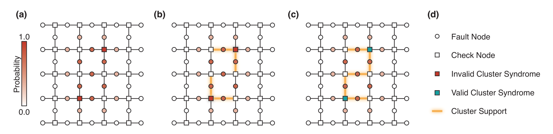
Figure 3 · Growth and merging of LSD clusters Source: hillmann2025, Fig. 2.
At sufficiently low physical error rates, typical cluster sizes do not grow with code size. This allows relatively large values of \(\mu\), even up to 20. In the relevant bivariate bicycle (BB) code tests, LSD is generally faster than OSD and achieves lower logical error rates.
BF-OSD: best-first search within the valid solution space. The two methods above search in the coordinates of \(x\) under the constraint \(Hx=s\). However, all valid \(x\) form an affine space. Choosing coordinates for that space allows an unconstrained search directly within it.
Best-first ordered statistics decoding (BF-OSD) starts from an OSD-0 particular solution \(x_0\) and uses elimination to obtain a basis \(g_j\) for \(\ker H\) banfi2026. Every configuration satisfying \(Hx=s\) can be written as
\[x(T)=x_0\oplus\bigoplus_{j\in T}g_j.\]Candidate generation therefore stays within \(x_0+\ker H\). The generators \(g_j\) represent displacements that preserve the syndrome.
BF-OSD can be understood as a likelihood-first search, similar in form to Dijkstra’s shortest-path algorithm. The search begins with the empty set \(T=\varnothing\) and stores candidates in a priority queue. Each step extracts the highest-scoring generated candidate \(T\), checks whether it improves the best solution found so far, and generates \(T'=T\cup\{j\}\). Requiring \(j>\max T\), with \(\max\varnothing=0\), prevents duplicate generation of the same combination. Once the query budget is exhausted, the best configuration found is returned.
Personal view. Despite its innovative search framework, BF-OSD does not outperform LSD by a large margin. In my view, one possible reason is that path distances in Dijkstra’s algorithm grow monotonically under expansion, whereas likelihood here does not change monotonically as generators are added. If reaching the most likely configuration \(x\) from the initial guess \(x_0\) requires crossing an energy barrier, a finite query budget may prevent the search from passing through the low-scoring intermediate candidates. The optimal configuration may then never enter the priority queue.
Tesseract: A* and beam search
Tesseract is a search-based decoder designed for high accuracy. It combines A* with beam search and achieves very low logical flip rates across several circuit-level decoding problems compared in the paper beni2025. The tradeoff is greater search time and memory demand.
Let \(F\) be the set of currently selected mechanisms, and let \(s(F)\) be the detector vector that remains unexplained. \(s(F)=0\) means that the configuration explains all observations. With independent mechanism priors, the search objective is
\[\min_{F:\,s(F)=0}g(F),\qquad g(F)=\sum_{j\in F}\log\frac{1-p_j}{p_j}.\]Starting from \(F=\varnothing\), each step adds a new mechanism \(j\) and updates
\[\begin{aligned} F'&=F\cup\{j\},\\ s(F')&=s(F)+H_{\cdot j}\pmod2,\\ g(F')&=g(F)+\log\frac{1-p_j}{p_j}. \end{aligned}\]Expansion considers only mechanisms connected to the lowest-index remaining triggered detector, and uses ordering rules to avoid duplicates.
A* assigns each state the priority
\[f(F)=g(F)+h(F).\]Here, \(g(F)\) is the cost of mechanisms already selected, and \(h(F)\) is a lower-bound estimate of the cost needed to explain the remaining detectors. Tesseract constructs this estimate by summing appropriately apportioned detector repair costs, and explores states with smaller \(f(F)\) first.
The beam limits how far the search may deviate from its current progress. Let \(r(F)=\operatorname{wt}(s(F))\), and let \(r_{\min}\) be the smallest \(r\) among visited states. If
\[r(F)>r_{\min}+B,\]the state \(F\) is skipped. The beam parameter \(B\) controls the allowed deviation in the number of remaining triggered detectors. A* determines which states are explored first, while the beam controls how wide a search range is retained.
3. Machine learning decoders
Recurrent Transformer
The basic components of a Transformer decoder are embedding, attention, and a multilayer perceptron (MLP). Embedding maps detector or data-node inputs to feature vectors. Attention uses the inner product between node \(a\)’s query and node \(b\)’s key to determine how \(a\) aggregates \(b\)’s value information. Each node’s feature vector is then independently processed by the MLP.
QEC requires both spatial relationships and history across cycles to be processed. AlphaQubit uses a recurrent Transformer: the current cycle’s detector information is embedded and added to a hidden state, then spatial attention within that cycle updates the representation, carrying history forward from round to round bausch2024. GraphQEC instead uses linear attention along the time direction to process historical information hu2025.
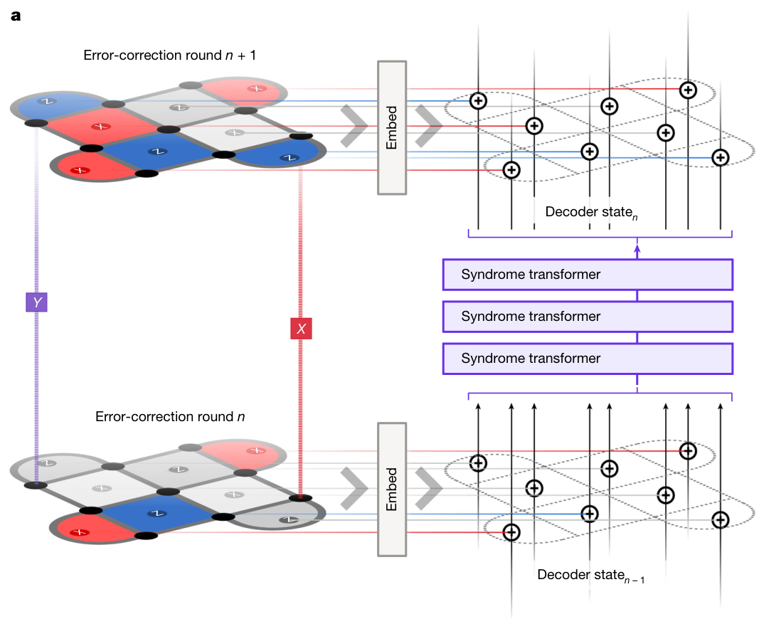
Figure 4 · AlphaQubit’s recurrent architecture Source: bausch2024, Fig. 2a.
These models ultimately predict logical flips. In AlphaQubit, for example, the readout maps detector hidden states to data-qubit representations, followed by pooling associated with the logical observable and an output stage. The Transformer approaches introduced here mainly use this logical readout, whereas configuration-based decoders output \(\hat x\) at the mechanism level.
CNN/GNN
Examples of this approach include Astra, which learns message-passing on the Tanner graph maan2025, and Cascade, which processes detector information through convolution and residual blocks gu2026. We will use Cascade as the example below.
A convolutional neural network (CNN) can be used for surface codes with regular local geometry. For nonlocal LDPC codes, a graph neural network (GNN) uses neighborhoods defined by Tanner graph adjacency.
First, for each spacetime detector \(v=(c,t)\), embed its observed value \(s_v\) as \(h_v^{(0)}\in\mathbb R^{D_h}\). We use \(D_h\) for the hidden dimension.
The features then pass through \(L\) bottleneck residual blocks. Each block first projects the features from \(D_h\) dimensions to \(D_h/4\), performs convolution in this lower-dimensional space, projects back to \(D_h\), and adds a residual connection. Batch normalization (BN) and sigmoid linear unit (SiLU) activation precede each projection or convolution.
During training, BN normalizes the activations in each feature channel over statistical dimensions including the batch, with learnable scale and bias. A residual connection adds the input back to the current block’s output, allowing the network to learn corrections to an existing representation.
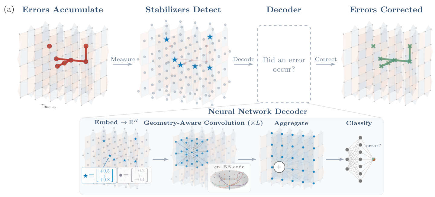
Figure 5 · Cascade architecture Source: gu2026, Fig. 1a.
Convolutional neighborhood aggregation can be written as
\[h_v'=W_{\mathrm{self}}h_v+\sum_{u\in\mathcal N(v)}W_{\delta(u,v)}h_u.\]Here, \(\delta(u,v)\) describes the relative geometry or connection relation. Connections with the same relation type share the same \(W_\delta\), so each edge does not need its own matrix. On a local surface-code graph, each layer expands the receptive field by only a constant amount. Propagating information over a distance-\(d\) scale therefore typically requires \(O(d)\) layers.
Finally, detector representations are mapped to data qubits, pooled over the logical operator support, and passed to an MLP that outputs logical flip probabilities.
Personal view. An output consisting only of the logical class does not provide all the information needed to distinguish data errors from measurement errors in the final few rounds. For example, consider an interior data qubit adjacent to two X-checks in a distance-\(d\) surface code. If both check measurements are wrong in the final round, the observations may be identical to those produced by a Z flip on that data qubit. Under the relevant noise model, the latter can even be the more likely explanation. A reliable Pauli frame therefore usually requires support from sufficiently many subsequent rounds. A decoder that outputs only the logical class cannot provide this timing information. Such an output is insufficient for a general fault-tolerant quantum computing architecture, motivating the online decoding discussed next.
4. Online decoders
Why do we need online decoding?
Two-qubit gate times, the number of gates per cycle, and the degree of parallelism together determine how quickly a physical platform generates detector data. To sustain QEC over long periods, the decoder’s amortized processing time must be shorter than the physical cycle time. Otherwise, undecoded data continually accumulate.
For example, the Gross \([[144,12,12]]\) code uses 144 data qubits and 144 measurement qubits. Its 144 weight-6 checks require \(144\times6=864\) two-qubit gates bravyi2024. Executing X- and Z-checks in separate groups gives an example 12-layer schedule with 72 parallel gates per layer. Google’s superconducting surface-code experiment reported 1.1 μs/cycle, which provides a reference timescale for superconducting platforms acharya2024.
Trapped-ion platforms have longer gate times. Quantinuum Helios has native two-qubit operations of approximately 70 μs ransford2026. Section 5 and Table 5 of the original Gross code paper give a 7-layer schedule, with a peak of 144 simultaneous gates under full parallelism. Estimating the entangling part of each controlled-NOT (CNOT) gate as one native \(R_{ZZ}(\pi/2)\) operation gives \(7\times70\,\mu\mathrm{s}=0.49\,\mathrm{ms}\), or 490 μs/cycle for the two-qubit operations alone. This budget extrapolates from Helios’s native gate duration. A complete QEC cycle must also include single-qubit rotations, transport, cooling, measurement, and reset. For neutral atoms, representative architectures have millisecond-scale QEC cycle budgets sunami2025.
Beyond throughput, we must consider when correction results can be committed. With measurement errors, one round of observations is generally insufficient to distinguish data errors from measurement errors, unless single-shot QEC is used. The newest round in a multi-round experiment faces the same issue: subsequent data are needed to determine the Pauli frame of earlier rounds.
In settings that typically require \(O(d)\) temporal redundancy, an additional wait of roughly \(d/2\) rounds gives a sense of the latency scale. An online decoder must therefore both keep pace with detector data and continuously output committable Pauli frame updates within a finite latency.
Sliding window decoding
Sliding windows are a common approach to online decoding skoric2023. Assume that the Pauli frame at the initial boundary is known, and take a window containing \(R=2d\) rounds. The first \(d\) rounds form the commit region, and the last \(d\) form a buffer that provides additional measurement information for earlier rounds. The end of the buffer lacks subsequent observations to rule out measurement errors, so Pauli frame estimates in the buffer are not committed.
Each time, decode the entire window but commit corrections only for the first \(d\) rounds. Then shift the window forward by \(d\) rounds, update the boundary using the committed results, and repeat. Decoding can thus proceed continuously as detector data arrive.
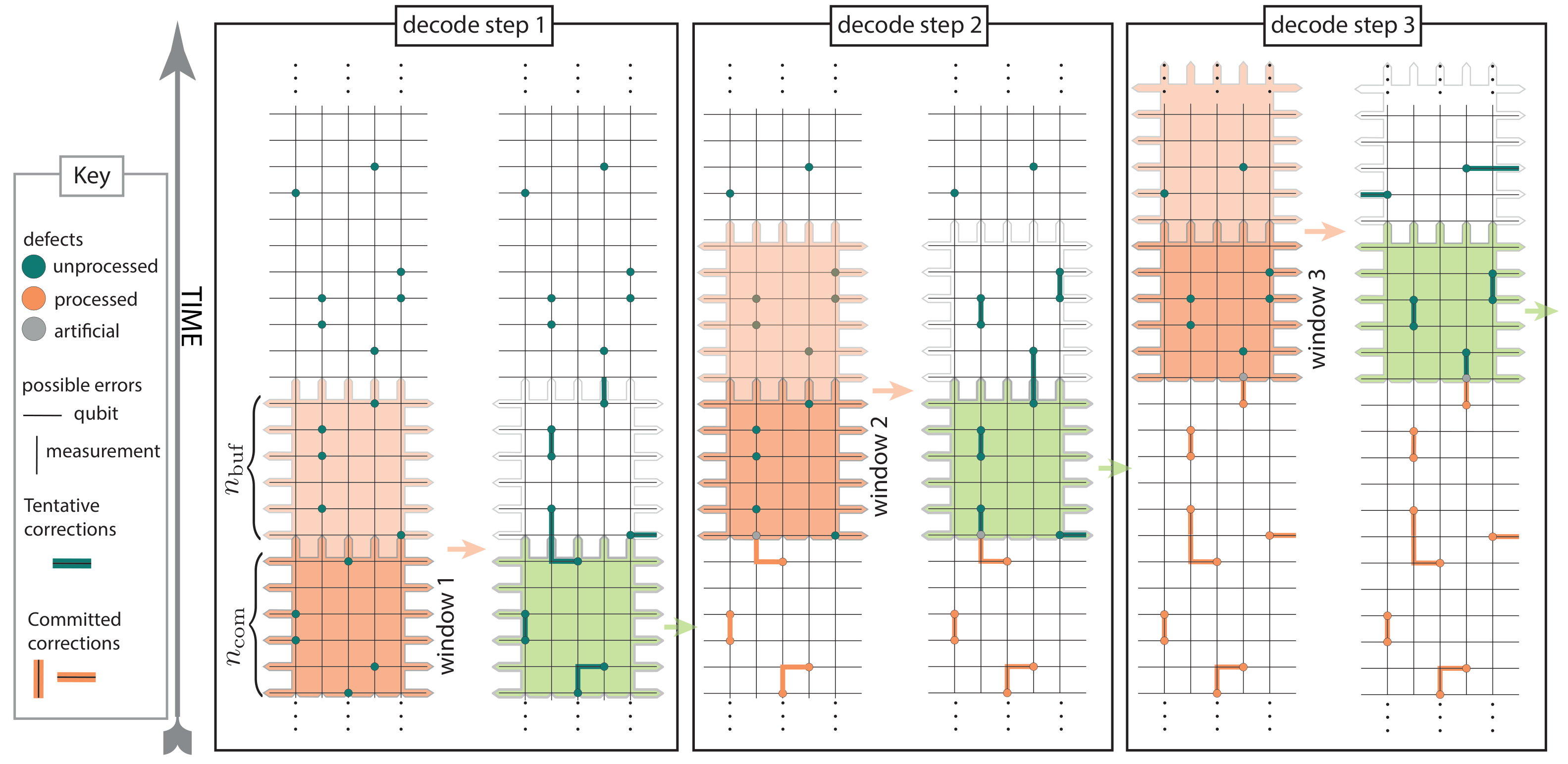
Figure 6 · Sliding window commit region and buffer Source: skoric2023, Fig. 2. Here, \(R=2d\) and committing \(d\) rounds at a time are example settings.
With sufficient computational resources, parallel window decoding can be used. The first layer splits the time series into multiple windows, decoding them in parallel and committing each window’s middle region under the protection of buffers on both sides. A second layer uses these committed results as boundaries to process the remaining regions. This two-layer window structure distributes the decoding of a long time series across multiple workers skoric2023.